Just Go with the Flow: Self-Supervised Scene Flow Estimation

Himangi Mittal Brian Okorn David Held
Robotics Institute
Carnegie Mellon University

[Paper] [Arxiv Paper] [Code] [1-minute-video] [5-minute-video]

teaser — (Left) We use two self-supervised losses to learn scene flow on large unlabeled datasets. The "nearest neighbor loss" penalizes the distance between the predicted point cloud (green) and each predicted point's nearest neighbor in the second point cloud (red). To avoid degenerate solutions, we estimate the flow between these predicted points (green) in the reverse direction back to the original point cloud (blue) to form a cycle. The new predicted points from the cycle (purple) should align with the original points (blue) and the distance between these two set of points, forms our second self-supervised loss: "cycle consistency". (Right) For the NuScenes dataset, scene flow is computed between point cloud at time 't' (red) and 't+1' (green) and the transformed cloud in shown in (blue)

Abstract

When interacting with highly dynamic environments, scene flow allows autonomous systems to reason about the non-rigid motion of multiple independent objects. This is of particular interest in the field of autonomous driving, in which many cars, people, bicycles, and other objects need to be accurately tracked. Current state of the art methods require annotated scene flow data from autonomous driving scenes to train scene flow networks with supervised learning. As an alternative, we present a method of training scene flow that uses two self-supervised losses, based on nearest neighbors and cycle consistency. These self-supervised losses allow us to train our method on large unlabeled autonomous driving datasets; the resulting method matches current state-of-the-art supervised performance using no real world annotations and exceeds state-of-the-art performance when combining our self-supervised approach with supervised learning on a smaller labeled dataset.

Problem Definition

For the task of scene flow estimation, we have a temporal sequence of point clouds recorded from LiDAR: point cloud X as the point cloud captured at time (t) and point cloud Y captured at time (t+1). Each point p(i) = {x(i),f(i)} in point cloud (X) contains the Cartesian position of the point and features such as color, intensity, etc.

The scene flow between the two point clouds describes the movement of each Cartesian point x(i) in point cloud X to its corresponding position x(i)' in the scene described by point cloud Y.

Losses

Nearest Neighbor Loss
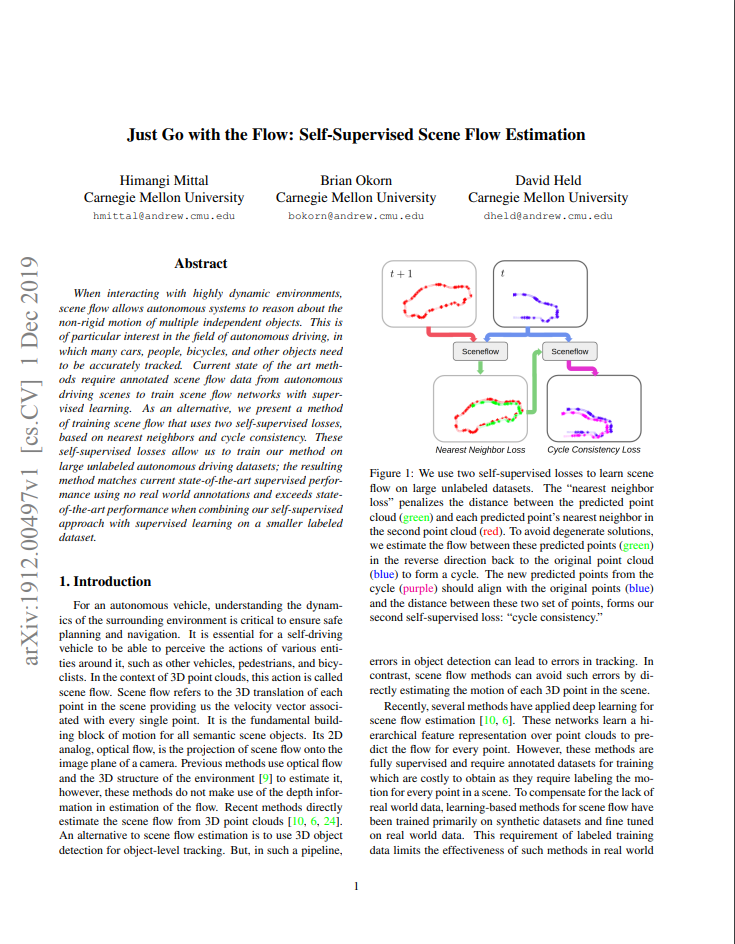
For large unlabeled datasets, since we do not have ground truth labels, we cannot compute the supervised loss. We use the nearest neighbor of our transformed point as an approximation for the true correspondence. For each transformed point in predicted point cloud, we find its nearest neighbor in Y and compute the Euclidean distance with that point.

Cycle Consistency Loss
To avoid degeneracies caused by cycle loss, we incorporate an additional self-supervised loss: cycle-consistency loss. We first estimate the forward flow to get a predicted point cloud. We then compute the scene flow in reverse direction under the cyclic assumption that the prediction of the reverse cycle should be similar to point cloud X.

Anchored Cycle Consistency Loss
In order to avoid unstable results and correct the structural distortions, we compute the anchored reverse flow by taking an average of prediction of foward cycle and point cloud Y.

Temporal Flip Augmentation
Having a dataset of point cloud sequences in only one direction may generate a motion bias. To reduce this bias, we augment the training set by temporally flipping the point clouds i.e. reversing the flow.

Experiments

Datasets Used : nuScenes and KITTI

Evaluation Metric : EPE, Acc1 (0.05), Acc2 (1.0)

Self-Supervised training on nuScenes
We begin with training our self-supervised model on nuScenes dataset using the combination of Nearest Neighbor Loss and Anchored Cycle loss. Since we wish to use Flownet3D as our scene flow estimation module, we initialize our network with Flownet3D weights pretrained on FlyingThing3D dataset.

Self-Supervised training on nuScenes and KITTI
Once the model has been trained on nuScenes, we fine-tune on KITTI in a self-supervised manner. For the comparison with the baseline, we use the Flownet3D model pretrained on FlyingThings3D without any fine-tuning on KITTI.

Supervised fine-tuning on KITTI
In order to evaluate the performance of our method on the real-world datasets having ground truth flow annotations, we fine tune our model on KITTI. For our method, we pretrain the model on nuScences using our self-supervised loss, and then introduce the KITTI data for supervised fine tuning. For the baseline, we use Flownet3d which is supervised fine tuned over the KITTI dataset. Both models are initialized with Flownet3D weights pretrained on FlyingThings3D.

Qualitative results

Scene flow estimation between point cloud at time 't' (red) and 't+1' (green) from KITTI dataset trained without any labeled lidar data. Our self-supervised method, trained on nuScenes and fine tuned on KITTI using self-supervised loss shown in (blue) and baseline training method, with no fine tuning, is shown in (purple). All models are pretrained on FlyingThings3D using a supervised loss. In the absence of any lidar annotations, our method clearly outperforms the baseline method, which over estimate the flow in many regions. (Best viewed in color)

Comparison of our self-supervised method vs baseline on unannotated nuScenes dataset. Scene flow is computed between point cloud at time 't' (red) and 't+1' (green) and the transformed cloud in shown in (blue). In our method, the predicted point cloud has a much better overlap with the point cloud of the next timestamp as compared to the baseline. Since nuScenes dataset does not provide any scene flow annotation, the supervised approaches cannot be fined tuned to this environment.

Improved scene flow estimation on annotated lidar data from the KITTI dataset between point clout at time 't' (red) and 't+1' (green). Our method, which is fine tuned on nuScenes using the self-supervised loss and KITTI using a supervised loss is shown in (blue). The baseline method is fine tuned only on KITTI using a supervised loss and is shown in (purple). While in aggregate, both methods well estimate the scene flow, the augmented training method (blue) is able to more closely match the next frame point cloud (green). In several of the cropped scenes, the purely supervised method (purple) underestimates the flow, staying too close to the initial point cloud (red). (Best viewed in color)

Comparison of levels of supervision on KITTI dataset. The nearest neighbor + anchored cycle loss is used for nuScenes (self-supervised) and KITTI (self-supervised).

Code

Code is available here.

Acknowledgments

This work was supported by the CMU Argo AI Center for Autonomous Vehicle Research.